A Simple Monte Carlo Program
首先,让我们从实现一个最简单的蒙特卡洛程序开始。
有两种随机性算法:蒙特卡洛和拉斯维加斯。随机算法在计算中使用了一定程度的随机性。拉斯维加斯(LV)随机算法总是产生正确的结果,而蒙特卡洛(MC)算法可能会产生正确的结果——但经常出错!但对于像光线追踪这样特别复杂的问题,我们可能不会将完美准确性放在首位,而是更注重在合理时间内得到一个答案。LV算法最终会得到正确结果,但我们无法保证需要多长时间才能得到结果。LV算法的经典例子是快速排序算法。快速排序算法总能完成一个完全排序的列表,但完成所需的时间是随机的。另一个LV算法例子是我们用来在单位球体中选取随机点的代码:
1
2
3
4
5
6
7
8
9
10
inline vec3 randomVectorOnUnitSphere()
{
    while (true)
    {
        if (point3 p = vec3::randomVector(-1, 1); p.lengthSquared() < 1)
        {
            return unitVectorLength(p);
        }
    }
}
这段代码能够最终返回一个位于单位球体中的随机点,但是我们无法预估该函数所需要的时间,也就是说,需要循环的次数是不确定的。然而,蒙特卡洛程序会给出一个结果的统计估计,并且运行时间越长,估计值就会越精准。这意味着我们可以决定在某个时刻程序获得的结果足够精准并退出程序。
2.1 Estimating Pi
蒙特卡洛算法的一个经典例子是估算π的值,假设正方形之中内嵌了一个圆。
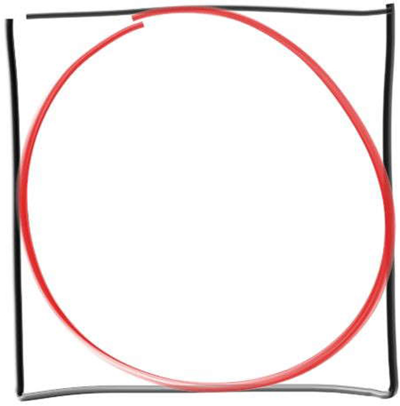
当我们在这个正方形上随机选择点时,位于圆内的点的比例应该等于圆的面积与正方形面积的比值,也就是: \(\frac{\pi r^2}{(2r)^2} = \frac{\pi}{4}\) 让我们在计算机中还原这个过程,并让该圆的半径为1,圆心在原点上:
1
2
3
4
5
6
7
8
9
10
11
12
13
14
15
16
17
18
19
20
21
22
#include "rayTracing.h"

#include <iostream>
#include <iomanip>
#include <math.h>
#include <stdlib.h>

int main()
{
    int N = 1000000;
    int insideCircle = 0;
    for (int i = 0; i < N; i++)
    {
        double x = randomDouble(-1, 1);
        double y = randomDouble(-1, 1);
        if (x * x + y * y) < 1
            insideCircle++;
    }

   std::cout << std::fixed<<std::setprecision(12);
   std::cout << "Estimate of Pi = " << (4.0 * insideCircle) / N << "\n";
}
运行这段程序,我们就可以结算得到一个π的近似值。
2.2 Showing Convergence
我们也可以将程序设定为一直运行,并按照一定频率返回π的估值。我们可以看到,随着有运行时间的变长,计算得到的π的值的误差也越来越小,也就是说,函数是在收敛的。
1
2
3
4
5
6
7
8
9
10
11
12
13
14
15
16
17
18
19
20
21
22
23
24
#include "rayTracing.h"

#include <iostream>
#include <iomanip>
#include <math.h>
#include <stdlib.h>

int main()
{
    int insideCircle = 0;
    int runs = 0;
    std::cout << std::fixed << std::setprecision(12);
    while(true)
    {
        runs++;
        double x = randomDouble(-1, 1);
        double y = randomDouble(-1, 1);
        if (x * x + y * y) < 1
            insideCircle++;

        if (runs % 100000 == 0)
            std::cout << "Estimate of Pi = " << (4.0 * insideCircle) / N << "\n";
    }
}
2.3 Stratified Samples(Jittering)
我们从上面这段代码返回的结果可以看出,在程序运行的最开始,随着runs的增加,计算结果会快速地接近π。但同时,估计值越接近π,每次新增采样对于最终结果的影响也越来越小。这就是所谓的收益递减法则 law of diminishing returns,换句话说,每次新的采样结果对于估计结果的改善效果减少。
这就是蒙特卡洛方法的缺点之一:通过随机采样来估计π值,当采样数较少时,估计值变化较大;当采样数增加时,估计值变化减小,但每次新增采样的效果越来越不明显。
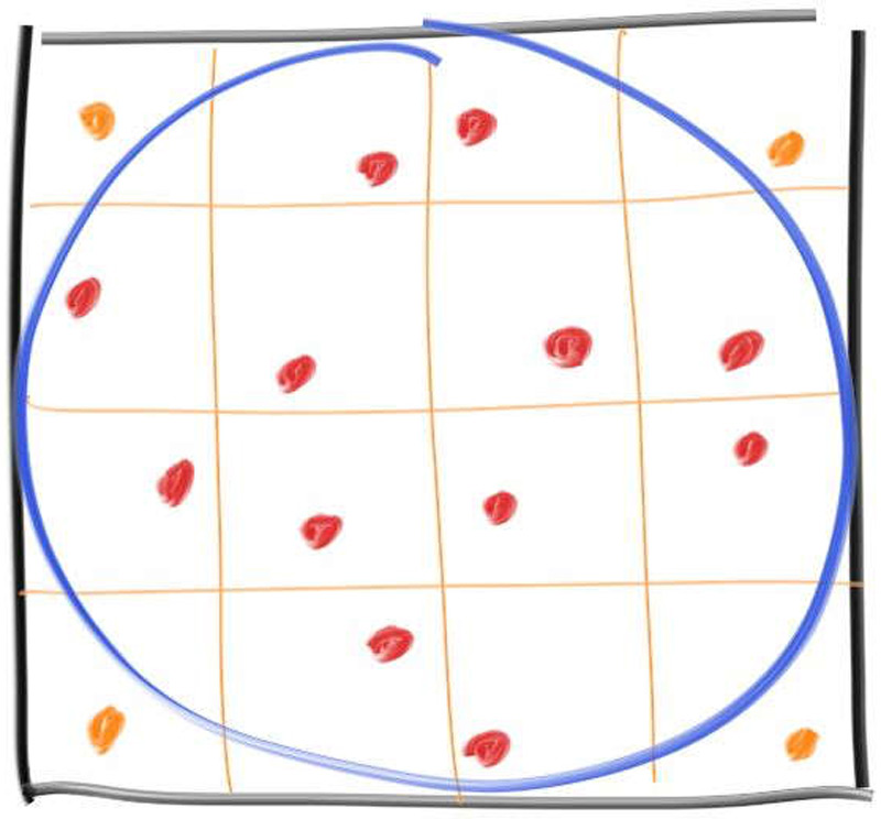
改进的方法是使用分层采样,也就是将采样的空间划分为多个小网格,然后在每个网格内进行一次采样,而不是完全随机采样,如下图所示。这种方法可以确保采样更均匀,减少估计误差
分层采样改变了样本的生成方式,但是我们需要提前知道采集了多少样本。我们以一百万个采样为例,并同时实现两种采样方式,这样便于我们比较两种方式之间的采样结果:
1
2
3
4
5
6
7
8
9
10
11
12
13
14
15
16
17
18
19
20
21
22
23
24
25
26
27
28
29
30
31
32
33
34
35
36
37
#include "rayTracing.h"

#include <iostream>
#include <iomanip>

int main()
{
	int insideCircle = 0;
    int insideCircleStratified = 0;
    int sqrtN = 1000;

    for (int i = 0; i < sqrtN; i++)
    {
        for (int j = 0; j < sqrtN; j++)
        {
            double x, y;
            // regular sampling
            x = randomDouble(-1, 1);
            y = randomDouble(-1, 1);
            if (x  * x + y * y < 1)
                insideCircle++;

            // stratified sampling
            x  = 2 * ((i + randomDouble()) / sqrtN) - 1;
            y  = 2 * ((j + randomDouble()) / sqrtN) - 1;
            if (x  * x + y * y < 1)
                insideCircleStratified++;
        }
    }

    std::cout << std::fixed << std::setprecision(12);
    std::cout
        << "Regular    Estimate of Pi = "
        << (4.0 * insideCircle) / (sqrtN * sqrtN) << '\n'
        << "Stratified Estimate of Pi = "
        << (4.0 * insideCircleStratified) / (sqrtN * sqrtN) << '\n';
}
最终我们可以得到一个结论,分层采样不仅可以有效减少估计结果的方差,还可以提高收敛速度。只是,这种优势会随着维度的提升而减小。这是因为高维空间中的样本均匀分布变得更加困难,且采样的复杂度显著增加。网格数量会随着维度的增加呈指数级增长,这显著增加了计算和存储的负载度。
我们来看一个具体的例子。假设我们在光线追踪中采样反射角度,那么我们可以将整个角度空间划分为多个子区域,并在每个子区域内进行采样。然而,如果考虑一个光线经过多次反射后在多个表面上的交点和角度,就需要在高维空间内进行分层采样,这使得分层采样的效率和效果迅速降低。这也是为什么在本系列博客中,我们不会对反射角进行分层。
在Ray Tracing The Rest Of Life系列博客中,我们将只是用康奈尔盒这一个场景,新的main.cpp如下:
1
2
3
4
5
6
7
8
9
10
11
12
13
14
15
16
17
18
19
20
21
22
23
24
25
26
27
28
29
30
31
32
33
34
35
36
37
38
39
40
41
42
43
44
45
46
47
48
49
50
51
52
53
54
55
56
#include "rayTracing.h"

#include "camera.h"
#include "hittableList.h"
#include "material.h"
#include "quad.h"
#include "sphere.h"

int main()
{
    hittableList world;

    auto red   = make_shared<lambertian>(color(.65, .05, .05));
    auto white = make_shared<lambertian>(color(.73, .73, .73));
    auto green = make_shared<lambertian>(color(.12, .45, .15));
    auto light = make_shared<diffuseLight>(color(15, 15, 15));

    // Cornell box sides
    world.add(make_shared<quad>(point3(555,0,0), vec3(0,0,555), vec3(0,555,0), green));
    world.add(make_shared<quad>(point3(0,0,555), vec3(0,0,-555), vec3(0,555,0), red));
    world.add(make_shared<quad>(point3(0,555,0), vec3(555,0,0), vec3(0,0,555), white));
    world.add(make_shared<quad>(point3(0,0,555), vec3(555,0,0), vec3(0,0,-555), white));
    world.add(make_shared<quad>(point3(555,0,555), vec3(-555,0,0), vec3(0,555,0), white));

    // Light
    world.add(make_shared<quad>(point3(213,554,227), vec3(130,0,0), vec3(0,0,105), light));

    // Box 1
    shared_ptr<hittable> box1 = box(point3(0,0,0), point3(165,330,165), white);
    box1 = make_shared<rotateY>(box1, 15);
    box1 = make_shared<translate>(box1, vec3(265,0,295));
    world.add(box1);

    // Box 2
    shared_ptr<hittable> box2 = box(point3(0,0,0), point3(165,165,165), white);
    box2 = make_shared<rotateY>(box2, -18);
    box2 = make_shared<translate>(box2, vec3(130,0,65));
    world.add(box2);

    camera camera;

    camera.aspectRatio = 1.0;
    camera.imageWidth = 600;
    camera.samplesPerPixel = 64;
    camera.maxDepth = 50;
    camera.background = color(0, 0, 0);

    camera.verticalFOV = 40;
    camera.lookFrom = point3(278, 278, -800);
    camera.lookAt = point3(278, 278, 0);
    camera.viewUp = vec3(0, 1, 0);

    camera.defocusAngle = 0;

    camera.render(world);
}
我们将分层采样应用在对每个像素位置周围的采样位置上:
1
2
3
4
5
6
7
8
9
10
11
12
13
14
15
16
17
18
19
20
21
22
23
24
25
26
27
28
29
30
31
32
33
34
35
36
37
38
39
40
41
42
43
44
45
46
47
48
49
50
51
52
53
54
55
56
57
58
59
60
61
62
63
64
65
66
67
68
69
70
71
72
73
74
75
76
77
78
class camera
{
public:
    ...

    void render(const hittable& world)
    {
        initialize();

        std::cout << "P3\n" << imageWidth << ' ' << imageHeight << "\n255\n";

        for (int j = 0; j < imageHeight; j++)
        {
            std::clog << "rScanlines remaining: " << (imageHeight - j) << "\n" << std::flush;

            for (int i = 0; i < imageWidth; i++)
            {
                color pixelColor = color(0, 0, 0);
                for (int sJ = 0; sJ < sqrtOfSamplesPerPixel; sJ++)
                {
                    for (int sI = 0; sI < sqrtOfSamplesPerPixel; sI++)
                    {
                        ray r = getRay(i, j, sI, sJ);
                        pixelColor += rayColor(r, maxDepth, world);
                    }
                }

                writeColor(std::cout, pixelColor * sampleScaleFactor);
            }
        }

        std::clog << "rDone.              \n";
    }

private:
    int imageHeight = 1;          // rendered image height in pixel count
    double sampleScaleFactor = 0; // color scale factor for a sum of pixel samples
    int sqrtOfSamplesPerPixel = 0;    // square root of number of samples per pixel
    double recipOfSqrt = 0;           // 1 / sqrtOfSamplesPerPixel
    ...

    void initialize()
    {
        imageHeight = static_cast<int> (imageWidth / aspectRatio);
        imageHeight = imageHeight < 1 ? 1 : imageHeight;

        sqrtOfSamplesPerPixel = static_cast<int> (sqrt(samplesPerPixel));
        sampleScaleFactor = 1.0 / (sqrtOfSamplesPerPixel * sqrtOfSamplesPerPixel);
        recipOfSqrt = 1.0 / sqrtOfSamplesPerPixel;

        ...
    }

    ray getRay(int i, int j, int sI, int sJ) const
    {
        // construct a camera ray originating from the aperture and
        // directed at random sampled point around the pixel location i, j
        // for stratified sample square sI, sJ

        vec3 offset = sampleFromSquareStratified(sI, sJ);
        point3 randomSampleLocation =
            firstPixelLocation + (i + offset.x()) * pixelDeltaU + (j + offset.y()) * pixelDeltaV;
        ...
    }

    vec3 sampleFromSquareStratified(int sI, int sJ) const
    {
        // return the vector to a random point in the square sub-pixel specified by grid
        // indices sI and sJ, for an idealized unit square pixel [-0.5,-0.5] to [+0.5,+0.5]

        double pX = (sI + randomZeroToOne()) * recipOfSqrt - 0.5;
        double pY = (sJ + randomZeroToOne()) * recipOfSqrt - 0.5;

        return {pX, pY, 0};
    }

    ...
};
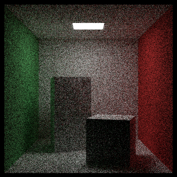
我们可以来比较一下不使用分层采样:
和使用分层采样之间结果的差异:
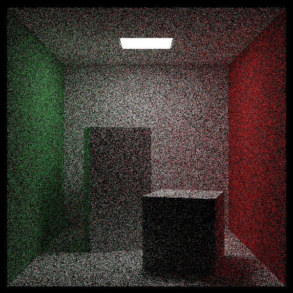
我们可以发现,使用分层采样后,方块的边缘以及平面的边缘都有了更为清晰的对比度。这是因为在我们当前的康奈尔盒中,使用的都是漫反射材质,且只有一个软光源,所以场景中的高信息密度的区域都集中在物体的边缘上。
我们将场景中光线变化的频率称为信息密度,高信息密度区域是那些光线变化快、细节多的地方,比如物体的边缘、表面细节、反射区域等。在这些区域,光线的变化频率高,细节丰富,因此需要更多的采样来准确捕捉这些细节。如果在这些区域采样不足,渲染结果就会出现明显的噪声或锯齿。
分层采样在这种情况下的作用是确保在高信息密度区域内有足够的样本,以捕捉这些区域的复杂变化。通过分层采样,可以在整个场景中更加均匀地分布样本,而不是让大部分样本集中在低信息密度区域,这样可以更有效地减少噪声,提高图像的质量。